Email Sentiment Analysis Using Python & Microsoft Azure - Part 1

What does our e-mail Sent Items folder say about our demeanor?

Can we use this and other complementary data to possibly determine trends in happiness or sadness at work?

Photo by Sebastian Herrmann on Unsplash

This is Part 1 of a multi-part article.

Introduction

Admitting right off the bat, I’ll consider myself a “noob” when it comes to most things data related. I have a pretty extensive history in traditional datacenter and cloud infrastructure, but pretty fresh to working with data. Kaggle has pretty much been my best friend over the last 12 months.

With that said, I’ve been engulfing myself in as many studies as possible around where my skills are lacking — calculus refreshers, statistics, coding, data engineering concepts, etc. I’d like to think that one of the best ways to learn is to do, but to also document the process as I’m experiencing it. Also, making sure to keep it fun!

I have also included a link to the Notebook that I created while writing this story. Feel free to use and modify as you see fit!

Concept Background

For those of us who use e-mail regularly, we’ve all sent snarky emails a few times, or many times…or maybe every day.

• “Per my last email…”
• “Going forward, I would suggest…”
• “This is complete and utter s**t!”

Do these look vaguely familiar? For many, it’s easy to either intentionally or unintentionally display your current state of emotion through email. You might be growing tired of having to explain the same situation multiple times, maybe your e-mail is a reflection of your increasing burnout, or maybe your car died this morning and you’re just having a bad day.

No matter what the cause, the history of our e-mails could actually provide a useful view into our attitude within an organization.

The remainder of this article will be focused on leveraging Jupyter Notebooks, the Microsoft Azure Text Analytics API to provide the horsepower, and using Python to explore, clean and present the sentiment analysis results.

Of course, I’ll also be blurring or sanitizing certain data just to make sure I still have a job after this. :)

Development Environment

The core environment will consist of the following:

• Outlook Sent Items CSV Export
• Azure Text Analytics API
• Azure Notebooks (Jupyter Notebook)

For Python specifically, we’ll be using the following packages:

• Numpy
• Pandas
• MatPlotLib
• Azure AI Text Analytics

Now that we understand the basics of the tools we’ll be using, lets get to building!

Step 1 — Deploy Azure Text Analytics

Photo by Vladimir Anikeev on Unsplash

We first need to deploy an API instance for us to target in the remainder of this article. Navigate to https://portal.azure.com and sign in. If you don’t have an account you can access free trials/credits by creating a subscription using one of the following:

Azure Pass: https://www.microsoftazurepass.com/

VS Dev Essentials: https://visualstudio.microsoft.com/dev-essentials/

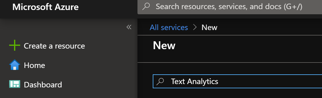
Once we’re logged in we’ll need to search for Text Analytics API.

• Click Create a resource.
• Type Text Analytics. Hit enter.
• Click Create.

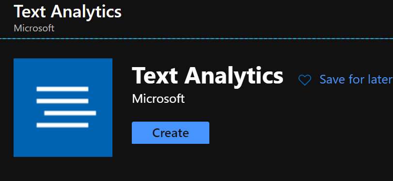
Create Text Analytics API instance

Next, we need to enter details about the service and its pricing tier. Type a Name, Subscription (if you have more than 1 active), Location (would recommend picking one close to you), Pricing Tier (F0 is free and works fine for this), and a Resource Group for it to live in. If you don’t have one, click Create New and give it a name.

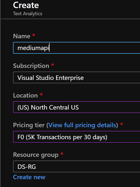
Azure Text Analytics API information

Once deployed, select All Resources from the left and click on your API resource. Then, click on Keys and Endpoint and copy the Endpoint and Key1 into a notepad or something for later use.

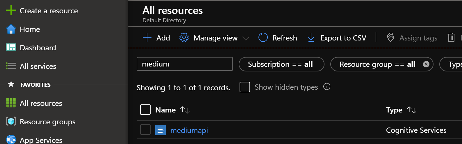
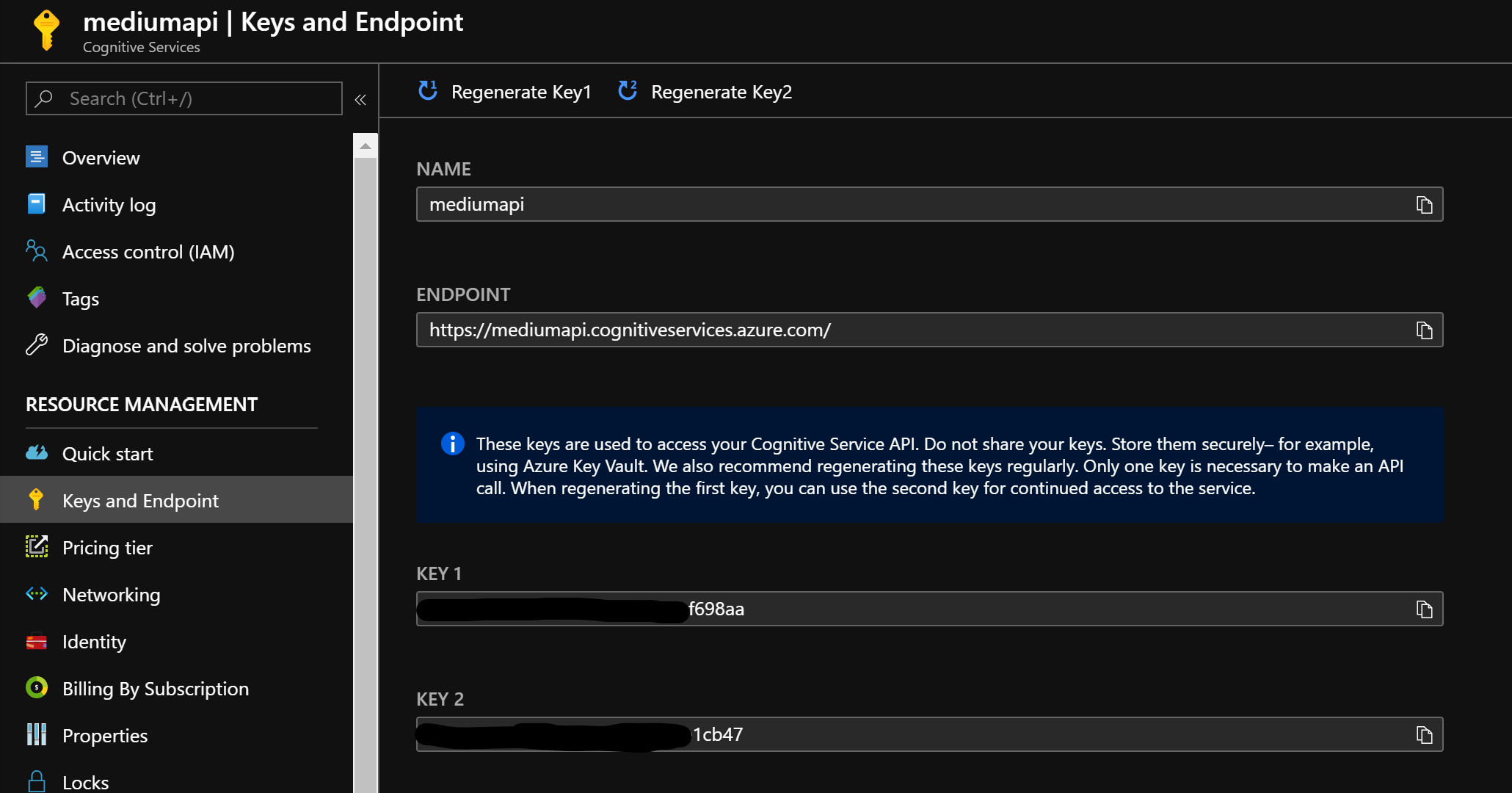
Key & Endpoint Retrieval

Step 2— Outlook CSV Export

Photo by Mika Baumeister on Unsplash

The next step is to grab a CSV export of your e-mail Sent Items. Considering we’re looking for our own personal sentiment scores, we’re only going to be concerned with our Sent Items.

• Open Outlook
• File → Open & Export → Import/Export
• Export to a file
• Comma Separated Values (CSV)
• Select your Sent Items folder
• Select an export location
• Finish the export

Step 3—Setup & Reviewing CSV Data

Photo by Kirill Pershin on Unsplash

Now that we have our CSV we need to start writing our code to explore and prepare our data for analysis. I would strongly recommend not opening the .csv file in Excel, as many of us refuse to organize or keep our mailbox clean. Instead, we’ll stick with loading it into a Pandas DataFrame.

We need to create a new Jupyter Notebook to work out of. I just called mine something simple like EmailSentiment.ipynb for now. If you don’t have Jupyter installed, and don’t want to use a hosted version, I would strongly suggest checking out Anaconda for a well-rounded package.

Now that we have our notebook we need to install the Azure Text Analytics API package for Python (if you don’t already have it).

!pip install azure-ai-textanalytics

We’re going to assume our dev environment already has Pandas and Numpy installed (both Anaconda and Azure Notebooks come with them available).

We can then continue to import the necessary packages. We’re also going to assign our Azure Text Analytics API key and endpoint information (from Step 1) into this cell.

import pandas as pd\
import numpy as np\
import matplotlib.pyplot as plt\
from matplotlib.pyplot import figure\
from azure.ai.textanalytics import TextAnalyticsClient\
from azure.core.credentials import AzureKeyCredential #Key and enpoint from Azure Text Analytics API service\
key = "324234k2j34i32j423423"\
endpoint = "<https://yourapi.cognitiveservices.azure.com/>"

We also need to define some functions we’re going to use later in our notebook. For organization sake, I just added both to a cell so they’re in the same location in the notebook.

We need one function to provide authentication for the Text Analytics API, as well as one for the core sentiment analysis. We’re following code from the following Quickstart in the Microsoft documentation but will make some modifications to the core function to fit our specific needs.

While the auth function is straight forward, we need to modify the sentiment analysis function to iterate over a list of lists (compared to a single hard-coded string), only retrieving the overall score(we’ll explore sentiment score ranges in the next post), and incrementing a frequency table we’ll create later.

#Creating the Azure authentication function\
def authenticate_client():\
    ta_credential = AzureKeyCredential(key)\
    text_analytics_client = TextAnalyticsClient(endpoint=endpoint, credential=ta_credential)\
    return text_analytics_client#Core function for running sentiment analysis\
#Modified to fit our specific needs\
#Added global variables we'll use later in this notebook\
def sentiment_analysis_example(client,list_name):\
    global senti_results\
    senti_results = {'Positive':0,'Neutral':0,'Negative':0,'Unknown':0}\
    global senti_errors\
    senti_errors = []\
    documents = list_name\
    for row in documents:\
        response = client.analyze_sentiment(documents = row)[0]\
        try:\
            if response.sentiment == "positive":\
                senti_results['Positive'] += 1\
            elif response.sentiment == "neutral":\
                senti_results['Neutral'] += 1\
            elif response.sentiment == "negative":\
                senti_results['Negative'] +=1\
            else:\
                senti_results['Unknown'] +=1\
        except:\
            senti_errors.append(row)\
    return(senti_results,senti_errors)#Assigning authentication function to object\
client = authenticate_client()

Now that we have our Azure API functions setup we’re ready to start exploring and preparing our dataset.

#Assign your filename to a variable\
emailFile = 'BenSent.CSV'#Display the first 5 rows of our CSV to inspect\
#Notice encoding --- this seemed to work for our CSV\
email_data = pd.read_csv(emailFile,encoding='ISO 8859--1')\
email_data.head()

If you run the above you should see something similar to the below output.

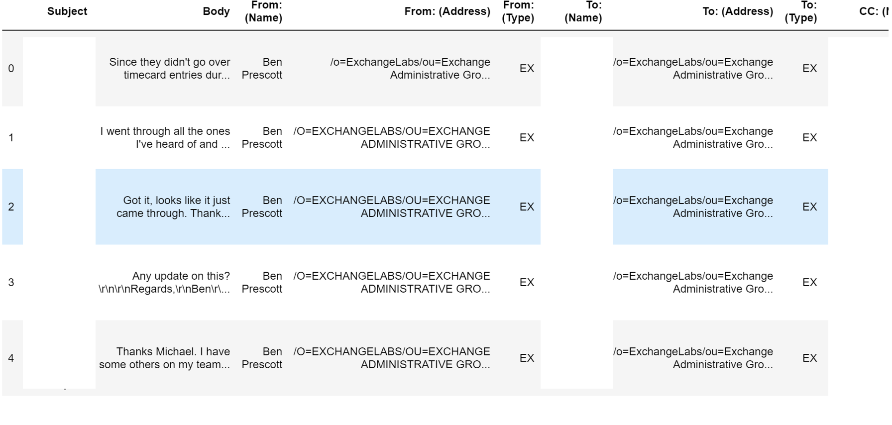
There are plenty of columns (useful or not) provided with the Outlook export, but you’ll find one critical data point missing — timestamps.

Unfortunately, Outlook doesn’t provide the ability to map the date/time property to the CSV export. For the sake of simplicity, we’re going to just analyze our dataset as a full batch. We’ll see how we can include dates in a follow-on post.

Step 4— Preparing The Dataset

Photo by Markus Spiske on Unsplash

Based on the available data in this scenario, we’ll focus on what we’re saying to others in our e-mails and determining if it was a positive, neutral or negative sentiment overall. We’re going to need to create a separate object with just the content from the Body column. We’ll do this using Pandas.

#Assign Body column to new object\
email_body = email_data['Body']#Display top 5 rows and the overall length of the series\
print(email_body.head())\
print('\n')\
print("Starting email count:",email_body.shape)

Here I’m using selection by column label considering we have those available to us. You can also use the column index, or whatever you prefer.

Now we can see we have just the body content, which is what we’ll use to perform sentiment analysis on. We’ll be closely monitoring the shape of our Series as we continue to clean this. We’re currently starting with 1675 rows.

Next, we’ll notice just from the first 5 rows that we have odd characters we don’t want to analyze, such as \ror \nand others. We’ll use a simple str.replace to remove these.

#Removing \r and \n characters from strings\
email_body = email_body.str.replace("\r","")\
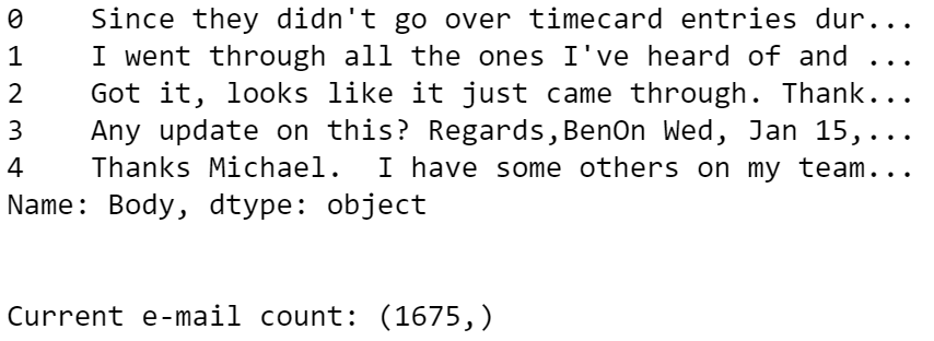
email_body = email_body.str.replace("\n","")#Display top 5 rows and the overall length of the series\
print(email_body.head())\
print('\n')\
print("Current e-mail count:",email_body.shape)

Next, we’re going to remove forwarded or trailing email threads where we don’t want to analyze a full email thread. An example is row index 3 where we see a date trailing my response in an e-mail thread.

I’ll clean these trailing e-mails by using what I know is automatically added to every sent item - my signature block. Using this as the target we can partition the data based on an identifying signature word(s) and trailing message into separate columns.

#Removing trailing email threads after start of my email signature\
split_df = email_body.str.partition("Regards")\
print(split_df[0:3])\
print('\n')\
print("Current e-mail count:",split_df.shape)

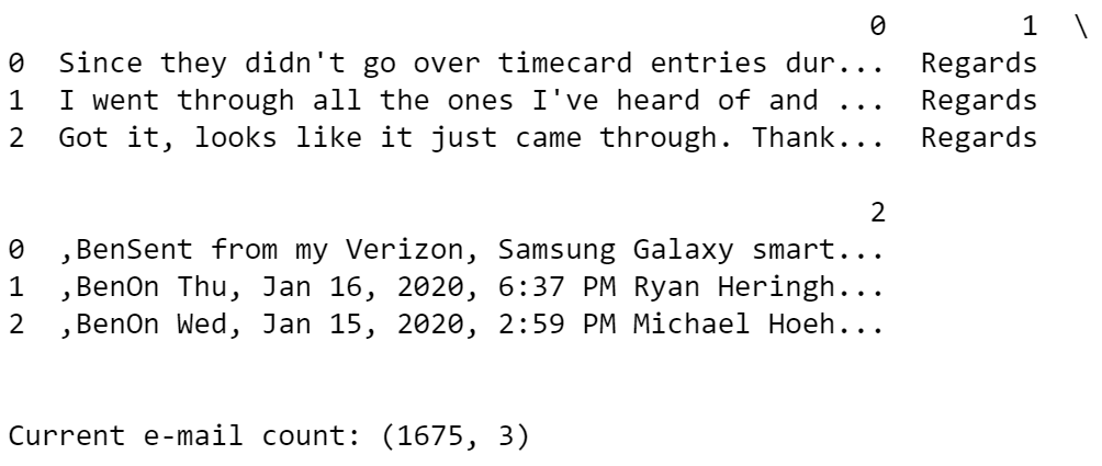
From the shape and output, we can now see we have 3 different partitioned columns — one for the email body content, one for the identified signature block word (“Regards” in my case) and one for the trailing message.

We now need to drop these additional columns and focus back on our body text. We’re also going to remove rows that are identified to have no information.

#Removing extra fluff from partitioning\
clean_col = split_df.drop(columns=[1,2]) #1 contains "Regards", 2 contains trailing text\
#Removing rows with NaN - no data\
clean_nan = clean_col.dropna()print("E-mail count before NaN removal:",clean_col.shape[0]) #Display before NaN removal\
print("E-mail count after NaN removal:",clean_nan.shape[0]) #Display before NaN removal

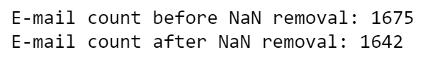
We can see before partitioning we had 1,675 rows. We dropped the two columns containing the fluff including and after my signature. After removing rows with NaN we are down to 1,642 emails. We need to continue cleaning by removing PTO emails and forwarded message emails. We’ll also add a column name to our body text column.

#Updating the primary column with name EmailBody\
clean_nan = clean_nan.rename(columns={0:"EmailBody"})#Remove emails with default out of office reply\
clean_pto = clean_nan[~clean_nan.EmailBody.str.contains("Hello,I am currently")]#Remove emails with a forwarded message\
cleaned_df = clean_pto[~clean_pto.EmailBody.str.contains("---------- Forwarded message ---------")]print("E-mail count before removals:",clean_nan.shape[0]) #Pre PTO count\
print("E-mail count after removing PTO messages:",clean_pto.shape[0]) #Post PTO count\
print("E-mail count after also removing forwarded messages:",cleaned_df.shape[0]) #Post fwd removal

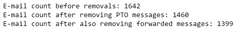
After checking the shape we can see we went from 1,642 rows to 1,460 rows, then finally to 1,399 rows. Keep in mind, we’re cleaning all of this to make sure our sentiment analysis returns as accurate information as possible.

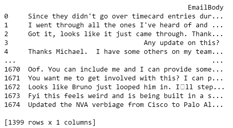
If we print the cleaned_df Series we’ll see that we have rows that look to be empty. We need to make sure we remove those so that our analysis doesn’t error out. We’ll do this by using Pandas’ df.replace and replace empty data with NaN.

#Considering we know we still have rows with no data, we'll replace the empty space with NaN\
#We can see all visible rows with nothing now show NaN\
cleaned_df['EmailBody'].replace(" ",np.nan,inplace=True)\
print(cleaned_df)

Now our empty rows will show NaN. We can now drop those rows by using pd.dropna() .

#We can now find all rows with NaN and drop them using pd.dropna\
cleaned_df = cleaned_df.dropna()\
print(cleaned_df)\
print('\n')\
print("E-mail count after dropping empty rows/rows with NaN:",cleaned_df.shape)

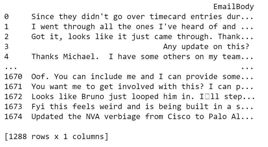
After removing our NaN rows were down to 1,288 rows. Feel free to continue exploring your data further to make sure you don’t have additional fluff that should be removed. While this won’t be perfect, we do want the results to be as legitimate as possible.

As for the last step, we’re going to convert our DataFrame into a list of lists that contains strings. We’ll use this to send to our API and return our results.

#Create an empty list to store values\
#Iterate over each row in the dataframe and append it to the listsenti_list = []for row in range((cleaned_df.shape[0])):\
    senti_list.append(list(cleaned_df.iloc[row,:]))

#Length of list matches length of old df\
print("E-mail count before error removal, ready for analysis:",len(senti_list))

We can print the length of the list of lists to make sure that it matches our DataFrame row count, which it does.

Step 5— Performing Sentiment Analysis

Photo by Tim Mossholder on Unsplash

Now that we have a list of “meh, I kind of cleaned it” data, we can start to send the data to our Azure API, retrieve the results, and visualize our data.

We’re going to provide our newly created list as our list_name argument in our core sentiment analysis function. The function is written in a way to provide not just a frequency table of results, but also a list containing the rows themselves that may contain errors when analyzing.

This next part may take a while depending on how many rows are being sent to the API. You may also find yourself having to scale your API service. If that is the case I would suggest trimming your list down for practice purposes.

#Trigger the sentiment analysis function, passing in our list of lists\
sentiment = sentiment_analysis_example(client,senti_list)

Once this is completed we can review the initial results.

print(senti_results)\
print("\n")\
print("Sentiment errors:",senti_errors)\
print("Error count:",len(senti_errors))

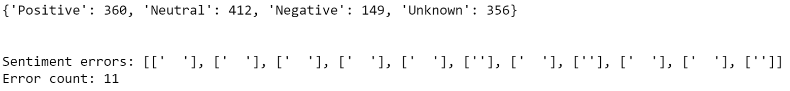
We can see two main things here: the overall sentiment results for our data and the rows that errored out when being analyzed. We can see we have a total of 11 rows not being analyzed and it seems to be because of varying white spaces.

We need to iterate over this list, iterate over our original dataset list of lists, and remove all lists containing these. We’ll also make a copy of our list of lists just so we have the historical version in case we need it in the future.

#Removing the errors from our list of lists\
#Assigning to a new variable so we have the unmodified original\
senti_cleaned = senti_listfor i in senti_errors:\
    for row in senti_cleaned:\
        if i == row:\
            senti_cleaned.remove(row)

print("E-mail count after removing error rows. Final used for analysis:",len(senti_cleaned))

We can see we’re down exactly 11 rows, which matches the count of errors. We can now re-run the analysis on our data copy to make sure we have no other errors.

#Triggering next run of analysis on the final dataset\
sentiment = sentiment_analysis_example(client,senti_cleaned)#Displaying the sentiment analysis results\
print(senti_results)\
print("\n")\
print("Sentiment errors:",senti_errors)\
print("Error count:",len(senti_errors))

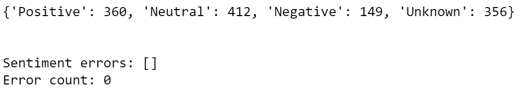
Reviewing the output we can verify we have no more errors (your mileage may vary) and are ready to move on to plotting our results.

Step 6— Visualization

Photo by Lukas Blazek on Unsplash

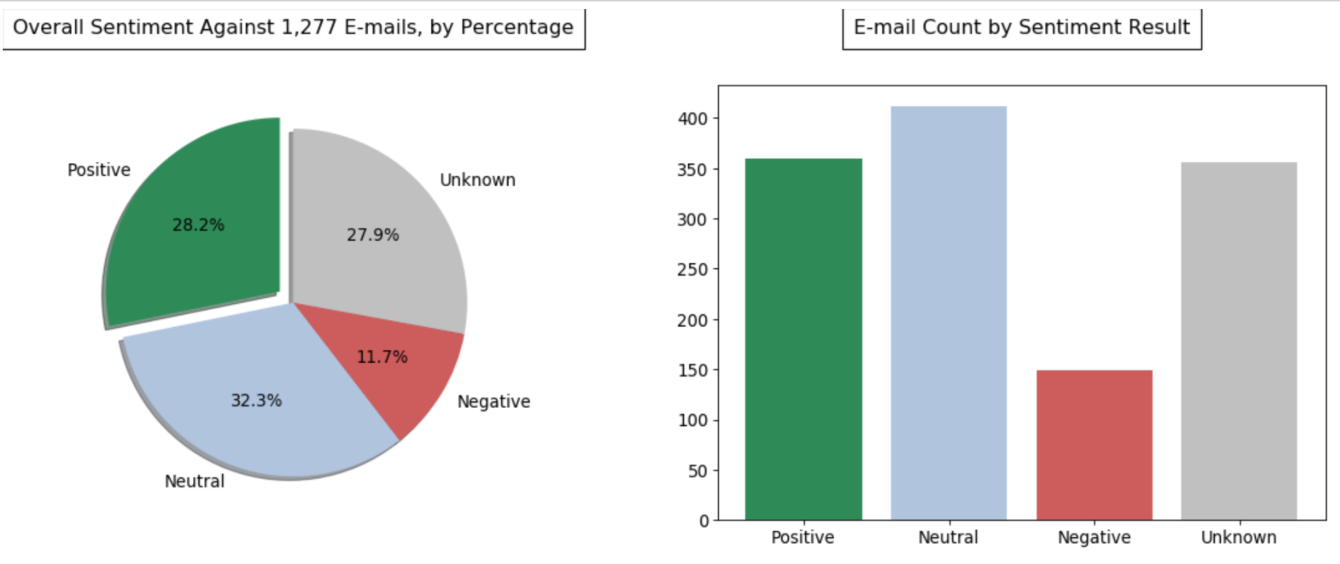
Now that we have our results in a nice dictionary we can work on plotting them into nice graphs. For this article, we’ll be focused on two views: overall sentiment percentage by result and e-mail count of each sentiment type.

To do this we’re going to use the matplotlib.pyplotlibrary. We’ll be creating both a pie chart (to visualize the percentages) and a bar chart (to visualize the e-mail count by result). We’ll also do some formatting changes to the plots before showing them, such as: color changes, font changes, padding/spacing, display sizes, etc.

#Setting our Key/Value pairs from our results\
keys = senti_results.keys()\
values = senti_results.values()#Establishing some format changes for our charts\
figure(num=None, figsize=(8,8),dpi=80)\
colors = ['seagreen','lightsteelblue','indianred','silver']\
explode = (0.1, 0, 0, 0)\
plt.rcParams.update({'font.size': 12})#Creating the first plot (pie chart)\
plt.subplot(221)\
plt.pie(values,labels=keys,colors=colors, explode=explode,autopct='%1.1f%%',shadow=True,startangle=90)\
plt.title('Overall Sentiment Against 1,277 E-mails, by Percentage',bbox={'facecolor':'1','pad':8},y=1.10)#Creating the second plot (bar chart)\
plt.subplot(222)\
plt.title('E-mail Count by Sentiment Result',bbox={'facecolor':'1','pad':8},y=1.10)\
plt.bar(keys,values,width=.8,color=colors)#Adjusting the spacing/padding between subplots\
plt.subplots_adjust(left=0.125, bottom=0.1, right=1.8, top=1.3, wspace=0.2, hspace=0.2)#Displaying the plots\
plt.show()

Now we can see we have a nice visual representation of our data! While we still have a bunch of “Unknown” response types from our API, we can tell that overall we aren’t as negative in our responses as we may have thought.

In some follow-on posts, we’ll look to break out each e-mails individual rating scores for each category and group them. We’ll also look to bring in some other data to compare/contrast with what we’ve found so far.

Hopefully, this post was useful or fun and you learned something along the way. Keep in mind, I’m very new to this and would definitely appreciate your feedback!