Peering Inside A Convolutional Neural Network

One hot topic in the field of deep learning is that of ‘model explainability’. In other words, being able to determine how an algorithm came up with the answers it did.

While we may understand what each layer in a neural network is using to activate the individual neurons, and the mathematical components behind how a neural network works, we still struggle to understand how it came up with certain information and what inputs triggered that information. For example, researchers have found that some networks are picking out relationships between features that weren’t explicitly provided to them.

Background

The thought behind this post is to train a convolutional neural network (CNN) and take a look at what it is ‘looking at’ to influence its predictions.

In traditional neural networks (i.e. dense or fully connected networks) we are able to follow a similar process, using the learned weights, biases, and neuron activation values as ways to see what each neuron in a layer recieved for input and its output activation.

However, CNNs are a bit more fun to look into, as they create feature maps from the input data, which allow us to visualize parts of an image that each feature map ‘sees’. More on this later…

Basic Concept of Fully Connected Networks

In dense (fully connected) neural networks we have an input layer, an output layer, and then some number of layers in between that have different activation functions and depths. The layers in between are called “hidden layers”, and many hidden layers typically make up a deep neural network.

Each hidden layer is made up of some defined number of neurons. Each neuron receives the input values and has an activation function (defined for the entire layer) that is ran against the input values to determine an output. Each connection to a node on each layer has a weight assigned to it. This weight is updated throughout the training process are part of the internal parameter tuning of the model, with the goal of achieving the best output. Finally, (typically) each node has a bias attached to it, providing an added influence to shift the output of the activation function.

Basic Concepts of Convolutional Networks

Convolutional networks work a bit differently, using convolutional layers and pooling layers to modify the input data as it moves through the network. Considering CNNs are commonly used in image processing tasks, the input values to a CNN are typically in a format commonly seen in images - length x width x color channels.

For example, you may have a set of images that are 150 pixels wide, by 150 pixels tall, with 3 color changes (Red, Green, Blue).

A convolutional layer performs a mathematical operation called a convolution. The TL;DR of this is that the layer takes input values and multiplies the elements against a 2D array of weights, called a filter (or kernel). The multipled values are then summed, creating a new output value.

See below for how a convolutional layer works. This is showcasing a 5x5 image with a dot product against a 3x3 filter/kernel.

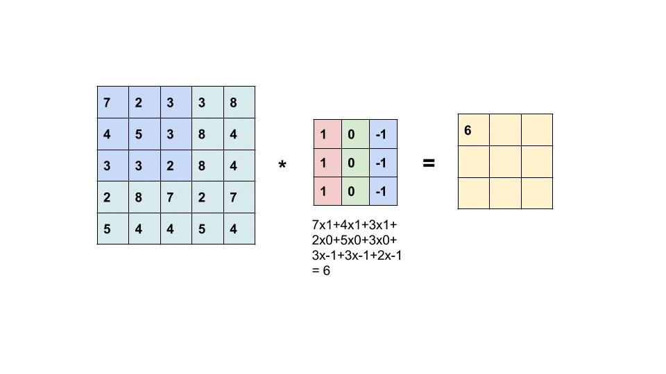
The result of this convolutional operation is what is called a feature map, which shows some learned representation of the input. However, as you can probably tell from the gif above, the output of the input and dot product of the filter is not the same shape as the original input. Each time we perform a convolution on an input the output is reduced in shape (shape being number of elements in each dimension - i.e. 50,50,3 for LxWxColors).

As our data progresses through the model each layer is creating a latent representation of the data, creating more and more feature maps from data of further and further reduced dimensionality. These feature maps are what we want to visualize to see what the network is identifying to represent each prediction.

Training A Basic CNN

We’ll keep this section short, as the entire post could be about training the network. For the full notebook please check this link.

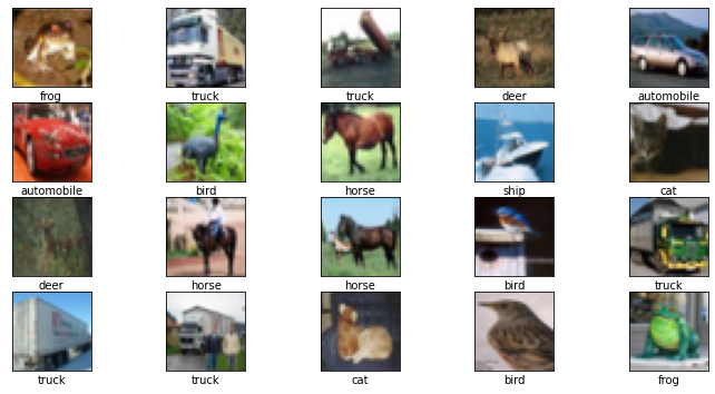
For simplicity sake we’re going to use the CIFAR-10 dataset. This dataset is easily imported through the TensorFlow Datasets library, consisting of 60,000 images across 10 categories (classes), each with dimensions of 32x32 with 3 color channels (RGB). In other words, the shape of our dataset will be (60000,32,32,3)

Make sure as you go through this to split it into a training and validation set, preferably tripartite with training/validation/test.

Lets load our training data into X and Y training variables, and X and Y testing variables.

# Load CIFAR-10 data from TensorFlow Datasets, adding to train/test sets
(x_train_full, y_train_full),(x_test, y_test)= cifar10.load_data()\

We can further split this to create a validation set by selecting a subset of the training data, as seen below:

x_train = x_train_full[:40000]
y_train = y_train_full[:40000]
x_val = x_train_full[40000:]
y_val = y_train_full[40000:]

We can also do some other Python magic and display some example images along with their Y values, converted to class names.

Considering neural networks work best with minimal variance in the data, I would also recommend scaling the input data. Its common to scale all pixel values in an image to between 0 and 1. This can be done easily by dividing each of your X variables by 255 (the highest pixel value in an image).

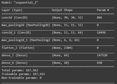
We can now create a basic CNN model, consisting of two convolutional layers, two maxpooling layers, a flattening operation to reduce dimensionality, and a fully connected layer prior to the output layer. In order for a dense (fully connected) layer to read this data it needs to be flattened into a single array.

We’re using sparse categorical crossentropy for our loss function, as we’re trying to predict an image’s class across 10 different options.

model3 = models.Sequential()
model3.add(Conv2D(32, kernel_size=(3,3),strides=(1,1), activation='relu', input_shape=(32,32,3)))
model3.add(MaxPool2D(2,2))
model3.add(Conv2D(64, kernel_size=(3,3),strides=(1,1), activation='relu'))
model3.add(MaxPool2D(2,2))
model3.add(Flatten())
model3.add(Dense(64, activation='relu'))
model3.add(Dense(10, activation='softmax'))

model3.summary()

earlystopcb = EarlyStopping(monitor='val_accuracy', patience=3)

model3.compile(loss = 'sparse_categorical_crossentropy',
              metrics = ['accuracy'],
              optimizer = 'Nadam')

We can also see how our model looks and what happens to our data’s shape as it moves through layers.

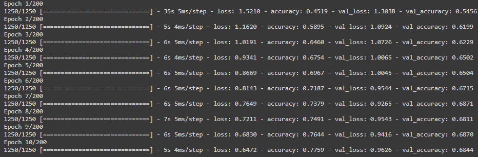
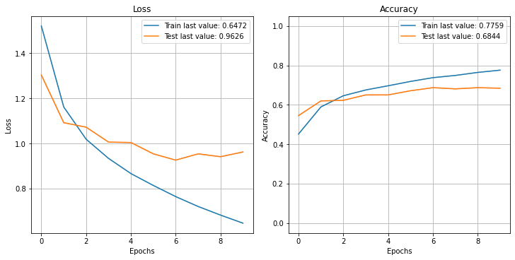
Now we can finally train our model. I’ve selected 200 epochs, but I’ve also included an early stopping callback, which will end the training if it notices no increase in validation data accuracy.

output3 = model3.fit(
    x_train_norm,
    y_train,
    epochs = 200,
    validation_data = (x_val_norm, y_val),
    callbacks=[earlystopcb] 
    )

The output shows the model reached about 68% accuracy on the validation data. Not very good, but good enough for the purpose of this post!

Generating Feature Maps

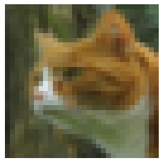
Now that we have a trained model that has its learned representations of the input dataset, we can pick an image to send for prediction and visualize the generated feature maps.

I randomly selected image #91 out of my X_test set, which happened to be a cat.

Now we want to grab our convolutional and max pooling layers from our trained model. We can do this by using a for loop or list comprehension, selecting the outputs of the first 4 layers.

Next, we define a new model that will generate those selected layer outputs, using the model’s input. Might sound kind of confusing, but we’re basically creating a new model from the existing model, mapping inputs and outputs.

# Extracts the outputs of the top 8 layers:
layer_outputs = [layer.output for layer in model3.layers[:4]]
# Creates a model that will return these outputs, given the model input:
activation_model = models.Model(inputs=model3.input, outputs=layer_outputs)

Now, lets run a prediction using this new model against our cat image!

activations = activation_model.predict(img_tensor)

Visualizing Feature Maps

Theres a whole block of code in how to pull out the images from the 4 layers we identified, so please reference the notebook. However, we can now use this predicted output to pull the activation values and visualize them, showing what the convolutional and pooling layers ‘saw’ as the data passed through them.

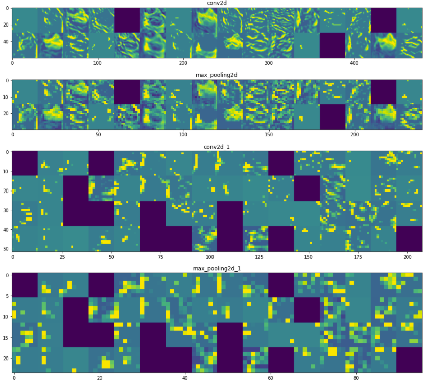
You can see how the pixelization of the image increases as it moves through convolutional/pooling layers, and we can see what each filter was ‘looking at’ on the cat to create the feature map. This is a similar concept to the activation values in a fully connected network, giving some insight into feature representation.

Keep in mind we aren’t trying to use this as a method of tuning the network, but rather trying to understand what the network used to make its decisions. Trying to find ways to provide “model explainability” will be critical in future growth and adoption in the machine learning space.

Note: The purple squares in the image are from my trained model that included dropout layers, which essentially force some nodes/filters to not activate in a layer. Its a form of regularization, but more on that in a future post. :)